AMM (Adaptive Multi Mode) optimizer

Adaptive Multi Mode · derivative-free black-box optimization
AMM reads your function with cheap probes, then routes the evaluation budget to the right classical algorithm, so one setting works across smooth, rugged and multimodal problems.
pip install amm-optimizerPyPI: 0.3.0 on PyPI (0.2.0 yanked).import numpy as npimport amm_optimizer
def rosenbrock(x): return float(np.sum(100 * (x[1:] - x[:-1] ** 2) ** 2 + (1 - x[:-1]) ** 2))
result = amm_optimizer.minimize( rosenbrock, x0=np.zeros(5), bounds=(-5, 5), budget=2000, seed=0, config=amm_optimizer.presets.get("c46"),)print(result.nfev, result.fun)print(result.x.round(3))2000 2.4585372370019567e-13[1. 1. 1. 1. 1.]The known optimum is x = (1, 1, 1, 1, 1) with f = 0. config= selects AMM (the frozen configuration
c46); without it minimize runs the original ATM sampler, which reaches only f = 1.7 on this example.
That output was produced by the frozen configuration c46 (config hash 2153948ebed51150) on 2026-10-22. Source and issues: https://github.com/BjBodner/amm-optimizer.
How it compares
Section titled “How it compares”On bbob instances that no design decision used (ids 101-110), AMM has the highest mean share of targets reached in 382 of 600 function, dimension and budget cells (64%, ties included). It is credibly behind some competitor in 35 (5.8%), and all 35 are listed on the limits page. It leads pycma IPOP-CMA-ES by +.12 to +.31 at every budget, and restarted SLSQP at every budget too, by +.015 [+.007, +.022] at 10 times the dimension, growing to +.302 [+.246, +.362] at 1000 times the dimension. The field is pycma IPOP and BIPOP, SLSQP, differential evolution, Optuna’s TPE, Nevergrad’s NGOpt and HCMA. The measure is the share of targets reached, 0 to 1.
This is the preregistered final test. The frozen configuration was run once on these instances. The analysis was run twice, as logged in advance: a first version without NGOpt at D 5 to 40 (still running then), and this one with every competitor at every dimension. “Credibly” is the rule fixed in advance: a competitor leads by more than 0.02 with posterior probability above 0.9 over the ten paired runs. The intervals behind it are about 25% too narrow, so these are counts and not significance statements. Every preregistered prediction for the final test held; the research log has them and the history of the analysis.
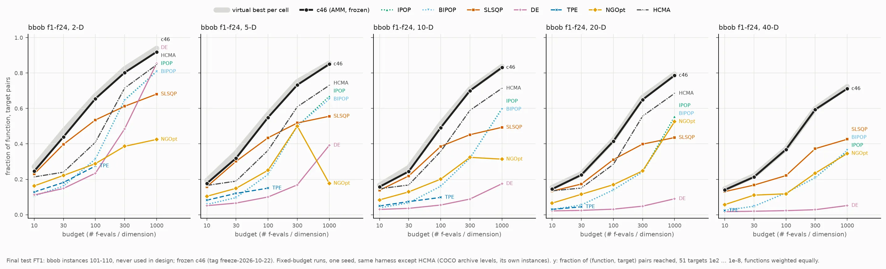
Reproduce this figure
- command
- final_ft1.py with no arguments, and ft1_plots.py as run for v2 (batch b095_final_ft1)
- seed
- 9000, one run per function, dimension, instance and budget (6,000 runs of AMM)
- instance ids
- 101-110, never used by any design decision
- budgets
- 10, 30, 100, 300, 1000 x D
- commit
- frozen configuration c46, config hash 2153948ebed51150 (the tagged history is in the research archive)
- competitors
- pycma IPOP/BIPOP, SLSQP, DE, TPE (capped slice) and NGOpt in the same harness; HCMA from the COCO archive
- hardware
- pending: filled from the run manifest
- cost
- pending: filled from the run manifest
- version
- 0.3.0
- config hash
- 2153948ebed51150
- licence
- Apache-2.0
- repository
- https://github.com/BjBodner/amm-optimizer
- PyPI
- 0.3.0 on PyPI (0.2.0 yanked)
- research archive DOI
- pendingpending
- checks
- local gate
tools/ci.py, 100% coverage, golden-master tests - preregistered
- yes, documents are in the research archive
What is in here
Section titled “What is in here”- Get started: install, a ten-line example, budget and bounds advice.
- How it works: the probes, the engines and the routing, with the routing map.
- Results: COCO-style ECDF per dimension and the cell-by-cell comparison.
- Limits and honesty: where AMM loses, what was tried, and what is not claimed.
- Reproduce and the research log: pinned versions, commands, preregistrations.
- Paper and cite.